External ballistics

Schlieren image of a bullet travelling in free-flight demonstrating the air pressure dynamics surrounding the bullet.

• External ballistics or exterior ballistics is the part of ballistics that deals with the behavior of a non-powered projectile in flight.

External ballistics is frequently associated with firearms, and deals with the unpowered free-flight phase of the bullet after it exits the barrel and before it hits the target, so it lies between transitional ballistics and terminal ballistics.

However, external ballistics is also concerned with the free-flight of rockets and other projectiles, such as balls, arrows etc.

Forces acting on the projectile

When in flight, the main forces acting on the projectile are gravity, drag, and if present, wind. Gravity imparts a downward acceleration on the projectile, causing it to drop from the line of sight. Drag, or the air resistance, decelerates the projectile with a force proportional to the square of the velocity. Wind makes the projectile deviate from its trajectory. During flight, gravity, drag, and wind have a major impact on the path of the projectile, and must be accounted for when predicting how the projectile will travel.

For medium to longer ranges and flight times, besides gravity, air resistance and wind, several meso variables described in the external factors paragraph have to be taken into account. Meso variables can become significant for firearms users that have to deal with angled shot scenarios or extended ranges, but are seldom relevant at common hunting and target shooting distances.

For long to very long ranges and flight times, minor effects and forces such as the ones described in the long range factors paragraph become important and have to be taken into account. The practical effects of these variables are generally irrelevant for most firearms users, since normal group scatter at short and medium ranges prevails over the influence these effects exert on firearms projectiles trajectories.

At extremely long ranges, artillery must fire projectiles along trajectories that are not even approximately straight; they are closer to parabolic, although air resistance affects this.

In the case of ballistic missiles, the altitudes involved have a significant effect as well, with part of the flight taking place in a near-vacuum.

Stabilizing non-spherical projectiles during flight

Two methods can be employed to stabilize non-spherical projectiles during flight:

• Projectiles like arrows or sabots like the M829 Armor-Piercing, Fin-Stabilized, Discarding Sabot (APFSDS) achieve stability by forcing their center of pressure (CP) behind their center of gravity (CG) with tail surfaces. The CP behind the CG condition yields stable projectile flight, meaning the projectile will not overturn during flight through the atmosphere due to aerodynamic forces.
• Projectiles like small arms bullets and artillery shells must deal with their CP being in front of their CG, which destabilizes these projectiles during flight. To stabilize such projectiles the projectile is spun around its longitudinal (leading to trailing) axis. The spinning mass makes the bullet's length axis resistant to the destabilizing overturning torque of the CP being in front of the CG.

Small arms external ballistics

Bullet drop and bullet path

Typical trajectory graph for a M4 carbine and M16A2 rifle using identical M855 cartridges with identical projectiles. Though both trajectories have an identical 25 m near zero, the difference in muzzle velocity of the projectiles gradually causes a significant difference in trajectory and far zero. The 0 inch axis represents the line of sight or horizontal sighting plane.

The effect of gravity on a projectile in flight is often referred to as bullet drop. It is important to understand the effect of gravity when zeroing the sighting components of a gun. To plan for bullet drop and compensate properly, one must understand parabolic shaped trajectories.

Bullet drop

In order for a projectile to impact any distant target, the barrel must be inclined to a positive elevation angle relative to the target. This is due to the fact that the projectile will begin to respond to the effects of gravity the instant it is free from the mechanical constraints of the bore. Thus, a bullet fired with a zero elevation angle can never impact a target higher than or at the same elevation as the center axis of the bore. The imaginary line down the center axis of the bore and out to infinity is called the line of departure and is the line on which the bullet leaves the barrel. As the bullet travels downrange, it arcs below the line of departure as it is being deflected off its initial path by gravity. Bullet drop is defined as the vertical distance of the projectile below the line of departure from the bore. Even when the line of departure is tilted upward or downward, bullet drop is still defined as the distance between the bullet and the line of departure at any point along the trajectory. Bullet drop is therefore of little practical use to shooters because it does not describe the actual trajectory of the bullet and is independent of the direction or distance to a target. It is best described as an intermediate parameter, most useful in ballistic computations where it is needed to calculate the values of other parameters. Apart from this, it is mainly useful when conducting a direct comparison of two different projectiles regarding the shape of their trajectories.

Bullet path

For hitting a distant target an appropriate positive elevation angle is required that is achieved by angling the line of sight from the shooter's eye through the centerline of the sighting system downward toward the line of departure. This can be accomplished by simply adjusting the sights down mechanically, or by securing the entire sighting system to a sloped mounting having a known downward slope, or by a combination of both. This procedure has the effect of elevating the muzzle when the barrel must be subsequently raised to align the sights with the target. A bullet leaving a muzzle at a given elevation angle follows a ballistic trajectory whose characteristics are dependent upon various factors such as muzzle velocity, gravity, and aerodynamic drag. This ballistic trajectory is referred to as the bullet path.

Bullet path is of great use to shooters because it allows them to establish ballistic tables that will predict how much elevation correction must be applied to the sight line for shots at various known distances. Bullet path values are determined by both the sight height, or the distance of the line of sight above the bore centerline, and the range at which the sights are zeroed, which in turn determines the elevation angle. A bullet following a ballistic trajectory has both forward and vertical motion. Forward motion is slowed due to air resistance, and in point mass modeling the vertical motion is dependent on a combination of the elevation angle and gravity. Initially, the bullet is rising with respect to the line of sight or the horizontal sighting plane. The bullet eventually reaches its apex (highest point in the trajectory parabola) where the vertical speed component decays to zero under the effect of gravity, and then begins to descend, eventually impacting the earth. The farther the distance to the intended target, the greater the elevation angle and the higher the apex.

The bullet path crosses the horizontal sighting plane two times. The point closest to the gun occurs while the bullet is climbing through the line of sight and is called the near zero. The second point occurs as the bullet is descending through the line of sight. It is called the far zero and defines the current sight in distance for the gun. Bullet path is described numerically as distances above or below the horizontal sighting plane at various points along the trajectory. This is in contrast to bullet drop which is referenced to the plane containing the line of departure regardless of the elevation angle. Since each of these two parameters uses a different reference datum, significant confusion can result because even though a bullet is tracking well below the line of departure it can still be gaining actual and significant height with respect to the line of sight as well as the surface of the earth in the case of a horizontal or near horizontal shot taken over flat terrain. Simply put, one parameter (bullet drop) compares the relative position of an actual bullet with an imaginary bullet that is not impeded by gravity while the other parameter (bullet path) describes the actual path of a bullet through the Earth's atmosphere, taking into account both gravity and aerodynamic effects.

Drag resistance modeling and measuring

Schlieren photo/Shadowgraph of the detached shock or bow shockwave around a bullet in supersonic flight, published by Ernst Mach in 1888.

Mathematical models for calculating the effects of drag or air resistance are quite complex and often unreliable beyond about 500 meters, so the most reliable method of establishing trajectories is still by empirical measurement.

Fixed drag curve models generated for standard-shaped projectiles

G1 shape standard projectile. All measurements in calibers/diameters.

Use of ballistics tables or ballistics software based on the Siacci/Mayevski G1 drag model, introduced in 1881, are the most common method used to work with external ballistics. Bullets are described by a ballistic coefficient, or BC, which combines the air resistance of the bullet shape (the drag coefficient) and its sectional density (a function of mass and bullet diameter).

The deceleration due to drag that a projectile with mass m, velocity v, and diameter d will experience is proportional to 1/BC, 1/m, v² and d². The BC gives the ratio of ballistic efficiency compared to the standard G1 projectile, which is a 1-pound (454 g), 1-inch (25.4 mm) diameter bullet with a flat base, a length of 3.28 inches (83.3 mm), and a 2-inch (50.8 mm) radius tangential curve for the point. The G1 standard projectile originates from the "C" standard reference projectile defined by the German steel, ammunition and armaments manufacturer Krupp in 1881. The G1 model standard projectile has a BC of 1. The French Gâvre Commission decided to use this projectile as their first reference projectile, giving the G1 name.

Sporting bullets, with a calibre d ranging from 0.177 to 0.50 inches (4.50 to 12.7 mm), have G1 BC’s in the range 0.12 to slightly over 1.00, with 1.00 being the most aerodynamic, and 0.12 being the least. Very-low-drag bullets with BC's ≥ 1.10 can be designed and produced on CNC precision lathes out of mono-metal rods, but they often have to be fired from custom made full bore rifles with special barrels.

Sectional density is a very important aspect of a bullet, and is the ratio of frontal surface area (half the bullet diameter squared, times pi) to bullet mass. Since, for a given bullet shape, frontal surface increases as the square of the calibre, and mass increases as the cube of the diameter, then sectional density grows linearly with bore diameter. Since BC combines shape and sectional density, a half scale model of the G1 projectile will have a BC of 0.5, and a quarter scale model will have a BC of 0.25.

Since different projectile shapes will respond differently to changes in velocity (particularly between supersonic and subsonic velocities), a BC provided by a bullet manufacturer will be an average BC that represents the common range of velocities for that bullet. For rifle bullets, this will probably be a supersonic velocity, for pistol bullets it will probably be subsonic. For projectiles that travel through the supersonic, transonic and subsonic flight regimes BC is not well approximated by a single constant, but is considered to be a function BC(M) of the Mach number M; here M equals the projectile velocity divided by the speed of sound. During the flight of the projectile the M will decrease, and therefore (in most cases) the BC will also decrease.

Most ballistic tables or software takes for granted that one specific drag function correctly describes the drag and hence the flight characteristics of a bullet related to its ballistics coefficient. Those models do not differentiate between wadcutter, flat-based, spitzer, boat-tail, very-low-drag, etc. bullet types or shapes. They assume one invariable drag function as indicated by the published BC.

Several drag curve models optimized for several standard projectile shapes are however available. The resulting fixed drag curve models for several standard projectile shapes or types are referred to as the:

G7 shape standard projectile. All measurements in calibers/diameters.

• G1 or Ingalls (flatbase with 2 caliber (blunt) nose ogive - by far the most popular)
• G2 (Aberdeen J projectile)
• G5 (short 7.5° boat-tail, 6.19 calibers long tangent ogive)
• G6 (flatbase, 6 calibers long secant ogive)
• G7 (long 7.5° boat-tail, 10 calibers tangent ogive, preferred by some manufacturers for very-low-drag bullets)
• G8 (flatbase, 10 calibers long secant ogive)
• GL (blunt lead nose)

How different speed regimes affect .338 calibre rifle bullets can be seen in the .338 Lapua Magnum product brochure which states Doppler radar established G1 BC data. The reason for publishing data like in this brochure is that the Siacci/Mayevski G1 model can not be tuned for the drag behavior of a specific projectile whose shape significantly deviates from the used reference projectile shape. Some ballistic software designers, who based their programs on the Siacci/Mayevski G1 model, give the user the possibility to enter several different G1 BC constants for different speed regimes to calculate ballistic predictions that closer match a bullets flight behavior at longer ranges compared to calculations that use only one BC constant.

The above example illustrates the central problem fixed drag curve models have. These models will only yield satisfactory accurate predictions as long as the projectile of interest has the same shape as the reference projectile or a shape that closely resembles the reference projectile. Any deviation from the reference projectile shape will result in less accurate predictions. How much a projectile deviates from the applied reference projectile is mathematically expressed by the form factor (i). The form factor can be used to compare the drag experienced by a projectile of interest to the drag experienced by the employed reference projectile at a given velocity (range). The problem that the actual drag curve of a projectile can significantly deviate from the fixed drag curve of any employed reference projectile systematically limits the traditional drag resistance modeling approach. The relative simplicity however makes that it can be explained to and understood by the general shooting public and hence is also popular amongst ballistic software prediction developers and bullet manufacturers that want to market their products.

More advanced drag models

Pejsa model

Besides the traditional drag curve models for several standard projectile shapes or types other more advanced drag models exist. The most prominent alternative ballistic model is probably the model presented in 1980 by Dr. Arthur J. Pejsa. Mr. Pejsa claims on his website that his method was consistently capable of predicting (supersonic) rifle bullet trajectories within 2.5 mm (0.1 in) and bullet velocities within 0.3 m/s (1 ft/s) out to 914 m (1,000 yd) when compared to dozens of actual measurements. The Pejsa model is a closed-form solution that does not need to use any tables or fixed drag curves generated for standard-shaped projectiles.

The greatest strength of the Pejsa model is that any projectile within a given flight regime (for example the supersonic flight regime) can be mathematically modeled well with only two velocity measurements a distance between said velocity measurements and a slope or deceleration constant factor. The model allows the drag curve to change slopes or curvature at three different points. Down range velocity measurement data can be provided around key inflection points allowing for more accurate calculations of the projectile retardation rate. The Pejsa model allows the slope factor to be tuned to account for subtle differences in the retardation rate of different bullet shapes and sizes. It ranges from 0.1 (flat-nose bullets) to 0.9 (very-low-drag bullets). If this slope or deceleration constant factor is unknown a default value of 0.5 will predict the flight behavior of most modern spitzer-type rifle bullets quite well. With the help of test firing measurements the slope constant for a particular bullet/rifle system/shooter combination can be determined. These test firings should preferably be executed at 60% and for extreme long range ballistic predictions also at 80% to 90% of the supersonic range of the projectiles of interest, staying away from erratic transonic effects. With this the Pejsa model can easily be tuned for the specific drag behavior of a specific projectile, making significant better (supersonic) ballistic predictions for ranges beyond 500 m (547 yd) possible. A practical downside of the Pejsa model is that accurate projectile specific down range velocity measurements to provide these better predictions can not be easily performed by the vast majority of shooting enthusiasts.

An average retardation coefficient can be calculated for any given slope constant factor if velocity data points are known and distance between said velocity measurements is known. Obviously this is true only within the same flight regime. With velocity actual speed is meant, as velocity is a vector quantity and speed is the magnitude of the velocity vector. Because the power function does not have constant curvature a simple chord average cannot be used. The Pejsa model uses a weighted average retardation coefficient weighted at 0.25 range.The closer velocity is more heavily weighted. The retardation coefficient is measured in feet whereas range is measured in yards hence 0.25 * 3.0 = 0.75, in some places 0.8 rather than 0.75 is used. The 0.8 comes from rounding in order to allow easy entry on hand calculators. Since the Pejsa model does not use a simple chord weighted average, two velocity measurements are used to find the chord average retardation coefficient at midrange between the two velocity measurements points. In order to find the starting retardation coefficient Dr. Pejsa provides two separate equations in his two books. The first involves the power function. The second equation is identical to the one used to find the weighted average at R / 4; add N * (R/2) where R is the range in feet to the chord average retardation coefficient at midrange and where N is the slope constant factor. After the starting retardation coefficient is found the opposite procedure is used in order find the weighted average at R / 4; the starting retardation coefficient minus N * (R/4). In other words N is used as the slope of the chord line. Dr. Pejsa states that he expanded his drop formula in a power series in order to prove that the weighted average retardation coefficient at R / 4 was a good approximation. For this Dr. Pejsa compared the power series expansion of his drop formula to some other unnamed drop formula’s power expansion to reach his conclusions. The fourth term in both power series matched when the retardation coefficient at 0.25 range was used in Pejsa’s drop formula. The fourth term was also the first term to use N. The higher terms involving N where insignificant and disappeared at N = 0.36, which according to Dr. Pejsa was a lucky coincidence making for an exceedingly accurate linear approximation, especially for N’s around 0.36. If a retardation coefficient function is used exact average values for any N can be obtained because from calculus it is trivial to find the average of any integrable function. Dr. Pejsa states that the retardation coefficient can be modeled by C * V^N where C is a fitting coefficient which disappears during the derivation of the drop formula and N the slope constant factor. The retardation coefficient equals the velocity squared divided by the retardation rate A. Using an average retardation coefficient allows the Pejsa model to be a closed-form expression within a given flight regime.

In order to allow the use of a G1 ballistic coefficient rather than velocity data Dr. Pejsa provided two reference drag curves. The first reference drag curve is based purely on the Siacci/Mayevski retardation rate function. The second reference drag curve is adjusted to equal the Siacci/Mayevski retardation rate function at a projectile velocity of 2600 fps (792.5 m/s) using a .30-06 Springfield Cartridge, Ball, Caliber .30 M2 152 grains (9.8 g) rifle spitzer bullet with a slope or deceleration constant factor of 0.5 in the supersonic flight regime. In other flight regimes the second Pejsa reference drag curve model uses slope constant factors of 0.0 or -4.0. These deceleration constant factors can be verified by backing out Pejsa's formulas (the drag curve segments fits the form V^{(2 - N)} / C and the retardation coefficient curve segments fits the form V² / (V^{(2 - N)} / C) = C * V^N where C is a fitting coefficient). The empirical test data Pejsa used to determine the exact shape of his chosen reference drag curve and pre-defined mathematical function that returns the retardation coefficient at a given Mach number was provided by the US military for the Cartridge, Ball, Caliber .30 M2 bullet. The calculation of the retardation coefficient function also involves air density, which Pejsa did not mention explicitly. The Siacci/Mayevski G1 model uses the following deceleration parametrization (60 °F, 30 inHg and 67% humidity, air density ρ = 1.2254 kg/m³). Dr. Pejsa suggests using the second drag curve because the Siacci/Mayevski G1 drag curve does not provide a good fit for modern spitzer bullets. To obtain relevant retardation coefficients for optimal long range modeling Dr. Pejsa suggested using accurate projectile specific down range velocity measurement data for a particular projectile to empirically derive the average retardation coefficient rather than using a reference drag curve derived average retardation coefficient. Further he suggested using ammunition with reduced propellant loads to empirically test actual projectile flight behavior at lower velocities. When working with reduced propellant loads utmost care must be taken to avoid dangerous or catastrophic conditions (detonations) with can occur when firing experimental loads in firearms.

Some software developers offer commercial software which is based on the Pejsa drag model enhanced and improved with refinements to account for normally minor effects (Coriolis, gyroscopic drift, etc.) that come into play at long range. The developers of these Pejsa model derived programs applied enhancements to the original Pejsa algorithms, using iterative or recursive mathematic approaches for each segment of the retardation coefficient curve with a different slope factor N, for better valid ballistic predictions beyond 1,000 m (1,094 yd) where high powered very-low-drag rifle bullets tend to go transonic and eventually subsonic. These Pejsa model based programs may also allow the use of an average retardation coefficient derived from velocity data as Dr. Pejsa's original ballistic software did. Further these other Pejsa model based ballistic software developers may have arbitrary chosen different reference projectile, velocity and/or air density variables than Dr. Pejsa used to alter the mathematical drag function or make their software suitable to allow the use of a non G1 ballistic coefficient.

Manges model

Although not as well known as the Pejsa model, an additional alternative ballistic model was presented in 1989 by Colonel Duff Manges (U S Army Retired) at the American Defense Preparedness (ADPA) 11th International Ballistic Symposium held at the Brussels Congress Center, Brussels, Belgium, May 9–11, 1989. A paper titled "Closed Form Trajectory Solutions for Direct Fire Weapons Systems" appears in the proceedings, Volume 1, Propulsion Dynamics, Launch Dynamics, Flight Dynamics, pages 665-674. Originally conceived to model projectile drag for 120 mm tank ammunition, the novel drag coefficient formula has been applied subsequently to ballistic trajectories of center-fired rifle ammunition with results comparable to those claimed for the Pejsa model.

The Manges model uses a first principles theoretical approach that eschews "G" curves and "ballistic coefficients" based on the standard G1 and other similarity curves. The theoretical description has three main parts. The first is to develop and solve a formulation of the two dimensional differential equations of motion governing flat trajectories of point mass projectiles by defining mathematically a set of quadratures that permit closed form solutions for the trajectory differential equations of motion. A sequence of successive approximation drag coefficient functions is generated that converge rapidly to actual observed drag data. The vacuum trajectory, simplified aerodynamic, d'Antonio, and Euler drag law models are special cases. The Manges drag law thereby provides a unifying influence with respect to earlier models used to obtain two dimensional closed form solutions to the point-mass equations of motion. The third purpose of this paper is to describe a least squares fitting procedure for obtaining the new drag functions from observed experimental data. The author claims that results show excellent agreement with six degree of freedom numerical calculations for modern tank ammunition and available published firing tables for center-fired rifle ammunition having a wide variety of shapes and sizes.

A Microsoft Excel application has been authored that uses least squares fits of wind tunnel acquired tabular drag coefficients. Alternatively, manufacturer supplied ballistic trajectory data, or Doppler acquired velocity data can be fitted as well to calibrate the model. The Excel application then employs custom macroinstructions to calculate the trajectory variables of interest. A modified 4th order Runge-Kutta integration algorithm is used. Like Pejsa, Colonel Manges claims center-fired rifle accuracies to the nearest one tenth of an inch for bullet position, and nearest foot per second for the projectile velocity.

The Proceedings of the 11th International Ballistic Symposium are available through the National Defense Industrial Association (NDIA) at the website http://www.ndia.org/Resources/Pages/Publication_Catalog.aspx.

6 Degrees of Freedom (6 DoF) model

There are also advanced professional ballistic models like PRODAS available. These are based on 6 Degrees of Freedom (6 DoF) calculations. 6 DoF modelling needs such elaborate input, knowledge of the employed projectiles and long calculation time on computers that it is impractical for non-professional ballisticians and field use where calculations generally have to be done on the fly on mobile computing devices like (ruggedized) PDAs or smartphones with relatively modest computing power. 6 DoF is generally used by military organizations that study the ballistic behavior of a limited number of (intended) military issue projectiles. Calculated 6 DoF trends can be incorporated as correction tables in more conventional ballistic software applications.

Doppler radar-measurements

For the precise establishment of drag or air resistance effects on projectiles, Doppler radar-measurements are required. Weibel 1000e Doppler radars are used by governments, professional ballisticians, defence forces and a few ammunition manufacturers to obtain real world data of the flight behavior of projectiles of their interest. Correctly established state of the art Doppler radar measurements can determine the flight behavior of projectiles as small as airgun pellets in three-dimensional space to within a few millimetres accuracy. The gathered data regarding the projectile deceleration can be derived and expressed in several ways, such as ballistic coefficients (BC) or drag coefficients (C_d).

Doppler radar measurement results for a lathe-turned monolithic solid .50 BMG very-low-drag bullet (Lost River J40 .510-773 grain monolithic solid bullet / twist rate 1:15 in) look like this:

Range (m)	500	600	700	800	900	1000	1100	1200	1300	1400	1500	1600	1700	1800	1900	2000
Ballistic coefficient	1.040	1.051	1.057	1.063	1.064	1.067	1.068	1.068	1.068	1.066	1.064	1.060	1.056	1.050	1.042	1.032

The initial rise in the BC value is attributed to a projectile's always present yaw and precession out of the bore. The test results were obtained from many shots not just a single shot. The bullet was assigned 1.062 for its BC number by the bullet's manufacturer Lost River Ballistic Technologies.

Doppler radar measurement results for a Lapua GB528 Scenar 19.44 g (300 gr) 8.59 mm (0.338 in) calibre very-low-drag bullet look like this:

Mach number	0.000	0.400	0.500	0.600	0.700	0.800	0.825	0.850	0.875	0.900	0.925	0.950	0.975	1.000	1.025	1.050	1.075	1.100	1.150	1.200	1.300	1.400	1.500	1.600	1.800	2.000	2.200	2.400
Drag coefficient	0.230	0.229	0.200	0.171	0.164	0.144	0.141	0.137	0.137	0.142	0.154	0.177	0.236	0.306	0.334	0.341	0.345	0.347	0.348	0.348	0.343	0.336	0.328	0.321	0.304	0.292	0.282	0.270

This tested bullet experiences its maximum drag coefficient when entering the transonic flight regime around Mach 1.200.

General trends in drag or ballistic coefficient

In general, a pointed bullet will have a better drag coefficient (C_d) or ballistic coefficient (BC) than a round nosed bullet, and a round nosed bullet will have a better C_d or BC than a flat point bullet. Large radius curves, resulting in a shallower point angle, will produce lower drags, particularly at supersonic velocities. Hollow point bullets behave much like a flat point of the same point diameter. Bullets designed for supersonic use often have a slightly tapered base at the rear, called a boat tail, which reduces air resistance in flight. Cannelures, which are recessed rings around the bullet used to crimp the bullet securely into the case, will cause an increase in drag.

The transonic problem

When the velocity of a rifle bullet fired at supersonic muzzle velocity approaches the speed of sound it enters the transonic region (about Mach 1.2–0.8). In the transonic region, the centre of pressure (CP) of most bullets shifts forward as the bullet decelerates. That CP shift affects the (dynamic) stability of the bullet. If the bullet is not well stabilized, it can not remain pointing forward through the transonic region (the bullets starts to exhibit an unwanted precession or coning motion that, if not damped out, can eventually end in uncontrollable tumbling along the length axis). However, even if the bullet has sufficient stability (static and dynamic) to be able to fly through the transonic region and stays pointing forward, it is still affected. The erratic and sudden CP shift and (temporary) decrease of dynamic stability can cause significant dispersion (and hence significant accuracy decay), even if the bullet's flight becomes well behaved again when it enters the subsonic region. This makes accurately predicting the ballistic behavior of bullets in the transonic region very difficult. Further the ambient air density has a significant effect on dynamic stability during transonic transition. Though the ambient air density is a variable environmental factor, adverse transonic transition effects can be negated better by bullets traveling through less dense air, than when traveling through denser air. Because of this, marksmen normally restrict themselves to engaging targets within the supersonic range of the bullet used.

Research into guided projectiles

To circumvent the transonic problems encountered by spin stabilized projectiles small arms projectiles can theoretically be guided during flight. The Sandia National Laboratories announced in January 2012 it has researched and test fired 4 inch (102 mm) long prototype dart-like, self-guided bullets for small-caliber, smooth-bore firearms that could hit laser-designated targets at distances of more than a mile (about 2,000 meters). These projectiles are not spin stabilized and the flight path can be course adjusted with an electromagnetic actuator 30 times per second. The researchers also claim they have video of the bullet radically pitching as it exited the barrel and pitching less as it flies down range, a disputed phenomenon known to long-range firearms experts as “going to sleep.” Because the bullet’s motions settle the longer it is in flight, accuracy improves at longer ranges, Sandia researcher Red Jones said. “Nobody had ever seen that, but we’ve got high-speed video photography that shows that it’s true,” he said. Since Sandia is seeking a private company partner to complete testing of the prototype and bring a guided bullet to the marketplace the future of this technology remains uncertain.

Testing the predictive qualities of software

Due to the practical inability to know in advance and compensate for all the variables of flight, no software simulation, however advanced, will yield predictions that will always perfectly match real world trajectories. It is however possible to obtain predictions that are very close to actual flight behavior.

Empirical measurement method

Ballistic prediction computer programs intended for (extreme) long ranges can be evaluated by conducting field tests at the supersonic to subsonic transition range (the last 10 to 20% of the supersonic range of the rifle/cartridge/bullet combination). For a typical .338 Lapua Magnum rifle for example, shooting standard 16.2 gram (250 gr) Lapua Scenar GB488 bullets at 905 m/s (2969 ft/s) muzzle velocity, field testing of the software should be done at ≈ 1200–1300 meters (1312 - 1422 yd) under International Standard Atmosphere sea level conditions (air density ρ = 1.225 kg/m³). To check how well the software predicts the trajectory at shorter to medium range, field tests at 20, 40 and 60% of the supersonic range have to be conducted. At those shorter to medium ranges, transonic problems and hence unbehaved bullet flight should not occur, and the BC is less likely to be transient. Testing the predictive qualities of software at (extreme) long ranges is expensive because it consumes ammunition; the actual muzzle velocity of all shots fired must be measured to be able to make statistically dependable statements. Sample groups of less than 24 shots do not obtain statistically dependable data.

Doppler radar measurement method

Governments, professional ballisticians, defence forces and a few ammunition manufacturers can use Doppler radars to obtain precise real world data regarding the flight behavior of the specific projectiles of their interest and thereupon compare the gathered real world data against the predictions calculated by ballistic computer programs. The normal shooting or aerodynamics enthusiast, however, has no access to such expensive professional measurement devices. Authorities and projectile manufacturers are generally reluctant to share the results of Doppler radar tests and the test derived drag coefficients (C_d) of projectiles with the general public.

In January 2009 the Finnish ammunition manufacturer Lapua published Doppler radar test-derived drag coefficient data for most of their rifle projectiles. With this C_d data engineers can create algorithms that utilize both known mathematical ballistic models as well as test specific, tabular data in unison. When used by predictive software like QuickTARGET Unlimited, Lapua Edition or Lapua Ballistics the Doppler radar test-derived drag coefficient data can be used for more accurate external ballistic predictions.

Some of the Lapua-provided drag coefficient data shows drastic increases in the measured drag around or below the Mach 1 flight velocity region. This behavior was observed for most of the measured small calibre bullets, and not so much for the larger calibre bullets. This implies some (mostly smaller calibre) rifle bullets exhibited coning and/or tumbling in the transonic/subsonic flight velocity regime. The information regarding unfavourable transonic/subsonic flight behavior for some of the tested projectiles is important. This is a limiting factor for extended range shooting use, because the effects of coning and tumbling are not easily predictable and potentially catastrophic for the best ballistic prediction models and software.

Presented C_d data can not be simply used for every gun-ammunition combination, since it was measured for the barrels, rotational (spin) velocities and ammunition lots the Lapua testers used during their test firings. Variables like differences in rifling (number of grooves, depth, width and other dimensional properties), twist rates and/or muzzle velocities impart different rotational (spin) velocities and rifling marks on projectiles. Changes in such variables and projectile production lot variations can yield different downrange interaction with the air the projectile passes through that can result in (minor) changes in flight behavior. This particular field of external ballistics is currently (2009) not elaborately studied nor well understood.

Predictions of several drag resistance modelling and measuring methods

The method employed to model and predict external ballistic behavior can yield differing results with increasing range and time of flight. To illustrate this several external ballistic behavior prediction methods for the Lapua Scenar GB528 19.44 g (300 gr) 8.59 mm (0.338 in) calibre very-low-drag rifle bullet with a manufacturer stated G1 ballistic coefficient (BC) of 0.785 fired at 830 m/s (2723 ft/s) muzzle velocity under International Standard Atmosphere sea level conditions (air density ρ = 1.225 kg/m³), Mach 1 = 340.3 m/s), predicted this for the projectile velocity and time of flight from 0 to 3,000 m (0 to 3,281 yd):

Range (m)	0	300	600	900	1,200	1,500	1,800	2,100	2,400	2,700	3,000
Radar test derived drag coefficients method V (m/s)	830	711	604	507	422	349	311	288	267	247	227
Time of flight (s)	0.0000	0.3918	0.8507	1.3937	2.0435	2.8276	3.7480	4.7522	5.8354	7.0095	8.2909
Total drop (m)	0.000	0.715	3.203	8.146	16.571	30.035	50.715	80.529	121.023	173.998	241.735
G1 drag model method V (m/s)	830	718	615	522	440	374	328	299	278	261	248
Time of flight (s)	0.0000	0.3897	0.8423	1.3732	2.0009	2.7427	3.6029	4.5642	5.6086	6.7276	7.9183
Total drop (m)	0.000	0.710	3.157	7.971	16.073	28.779	47.810	75.205	112.136	160.739	222.430
Pejsa drag model method V (m/s)	830	712	603	504	413	339	297	270	247	227	208
Time of flight (s)	0.0000	0.3902	0.8479	1.3921	2.0501	2.8556	3.8057	4.8682	6.0294	7.2958	8.6769
Total drop (m)	0.000	0.719	3.198	8.129	16.580	30.271	51.582	82.873	126.870	185.318	260.968
G7 drag model method V (m/s)	830	713	606	508	418	339	303	283	265	249	235
Time of flight (s)	0.0000	0.3912	0.8487	1.3901	2.0415	2.8404	3.7850	4.8110	5.9099	7.0838	8.3369
Total drop (m)	0.000	0.714	3.191	8.109	16.503	30.039	51.165	81.863	123.639	178.082	246.968

The table shows that the traditional Siacci/Mayevski G1 drag curve model prediction method generally yields more optimistic results compared to the modern Doppler radar test derived drag coefficients (C_d) prediction method. At 300 m (328 yd) range the differences will be hardly noticeable, but at 600 m (656 yd) and beyond the differences grow over 10 m/s (32.8 ft/s) projectile velocity and gradually become significant. At 1,500 m (1,640 yd) range the projectile velocity predictions deviate 25 m/s (82.0 ft/s), which equates to a predicted total drop difference of 125.6 cm (49.4 in) or 0.83 mrad (2.87 MOA) at 50° latitude.

The Pejsa drag model closed-form solution prediction method, without slope constant factor fine tuning, yields very similar results in the supersonic flight regime compared to the Doppler radar test derived drag coefficients (C_d) prediction method. At 1,500 m (1,640 yd) range the projectile velocity predictions deviate 10 m/s (32.8 ft/s), which equates to a predicted total drop difference of 23.6 cm (9.3 in) or 0.16 mrad (0.54 MOA) at 50° latitude.

The G7 drag curve model prediction method (recommended by some manufacturers for very-low-drag shaped rifle bullets) when using a G7 ballistic coefficient (BC) of 0.377 yields very similar results in the supersonic flight regime compared to the Doppler radar test derived drag coefficients (C_d) prediction method. At 1,500 m (1,640 yd) range the projectile velocity predictions have their maximum deviation of 10 m/s (32.8 ft/s). The predicted total drop difference at 1,500 m (1,640 yd) is 0.4 cm (0.16 in) at 50° latitude. The predicted total drop difference at 1,800 m (1,969 yd) is 45.0 cm (17.7 in), which equates to 0.25 mrad (0.86 MOA).

External factors

Wind

Wind has a range of effects, the first being the effect of making the bullet deviate to the side. From a scientific perspective, the "wind pushing on the side of the bullet" is not what causes wind drift. What causes wind drift is drag. Drag makes the bullet turn into the wind, keeping the centre of air pressure on its nose. This causes the nose to be cocked (from your perspective) into the wind, the base is cocked (from your perspective) "downwind." So, (again from your perspective), the drag is pushing the bullet downwind making bullets follow the wind.

A somewhat less obvious effect is caused by head or tailwinds. A headwind will slightly increase the relative velocity of the projectile, and increase drag and the corresponding drop. A tailwind will reduce the drag and the bullet drop. In the real world pure head or tailwinds are rare, since wind seldom is constant in force and direction and normally interacts with the terrain it is blowing over. This often makes ultra long range shooting in head or tailwind conditions difficult.

Vertical angles

The vertical angle (or elevation) of a shot will also affect the trajectory of the shot. Ballistic tables for small calibre projectiles (fired from pistols or rifles) assume that gravity is acting nearly perpendicular to the bullet path. If the angle is up or down, then the perpendicular acceleration will actually be less. The effect of the path wise acceleration component will be negligible, so shooting up or downhill will both result in a similar decrease in bullet drop.

Often mathematical ballistic prediction models are limited to "flat fire" scenarios based on the rifleman's rule, meaning they can not produce adequately accurate predictions when combined with steep elevation angles over -15 to 15 degrees and longer ranges. There are however several mathematical prediction models for inclined fire scenarios available which yield rather varying accuracy expectation levels.

Ambient air density

Air pressure, temperature, and humidity variations make up the ambient air density. Humidity has a counter intuitive impact. Since water vapor has a density of 0.8 grams per litre, while dry air averages about 1.225 grams per litre, higher humidity actually decreases the air density, and therefore decreases the drag.

Long range factors

Gyroscopic drift (Spin drift)

Gyroscopic drift is an interaction of the bullets mass and aerodynamics with the atmosphere that it is flying in. Even in completely calm air, with no sideways air movement at all, a spin-stabilized projectile will experience a spin-induced sideways component. For a right hand (clockwise) direction of rotation this component will always be to the right. For a left hand (counterclockwise) direction of rotation this component will always be to the left. This is because the projectile's longitudinal axis (its axis of rotation) and the direction of the velocity vector of the center of gravity (CG) deviate by a small angle, which is said to be the equilibrium yaw or the yaw of repose. The magnitude of the yaw of repose angle is typically only fractions of a degree. Since rotating objects react by moving 90 degrees from the applied force for right-handed (clockwise) spinning bullets, the bullet's axis of symmetry points to the right and a little bit upward with respect to the direction of the velocity vector as the projectile rotates through its ballistic arc on a long range trajectory. As an effect of this small inclination, there is a continuous air stream, which tends to deflect the bullet to the right. Thus the occurrence of the yaw of repose is the reason for bullet drift to the right (for right-handed spin) or to the left (for left-handed spin). This means that the bullet is "skidding" sideways at any given moment, and thus experiencing a sideways component.

The following variables affect the magnitude of gyroscopic drift:

• Projectile or bullet length: longer projectiles experience more gyroscopic drift because they produce more lateral "lift" for a given yaw angle.
• Spin rate: faster spin rates will produce more gyroscopic drift because the nose ends up pointing farther to the side.
• Range, time of flight and trajectory height: gyroscopic drift increases with all of these variables.
• density of the atmosphere: denser air will increase gyroscopic drift.

Doppler radar measurement results for the gyroscopic drift of several US military and other very-low-drag bullets at 1000 yards (914.4 m) look like this:

Bullet type	US military M193 Ball	US military M118 Special Ball	Palma Sierra MatchKing	LRBT J40 Match	Sierra MatchKing	Sierra MatchKing	LRBT J40 Match	LRBT J40 Match
Projectile weight (in grain)	55 gr	173 gr	155 gr	190 gr	220 gr	300 gr	350 gr	419 gr
Projectile diameter (in inches and mm)	.223 in / 5.56 mm	.308 in / 7.62 mm	.308 in / 7.62 mm	.308 in / 7.62 mm	.308 in / 7.62 mm	.338 in / 8.59 mm	.375 in / 9.53 mm	.408 in / 10.36 mm
Gyroscopic drift (in inches and mm)	23.00 in / 584 mm	11.50 in / 292 mm	12.75 in / 324 mm	3.00 in / 76 mm	7.75 in / 197 mm	6.5 in / 165 mm	0.87 in / 22 mm	1.90 in / 48 mm

The table shows that the gyroscopic drift is rather variable and no clear trend is easily distinguishable.

Magnus effect

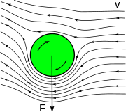
The Magnus effect. V represents the wind, the arrow F is the resulting Magnus force towards the side of lower pressure.

Spin stabilized projectiles are affected by the Magnus effect, whereby the spin of the bullet creates a force acting either up or down, perpendicular to the sideways vector of the wind. In the simple case of horizontal wind, and a right hand (clockwise) direction of rotation, the Magnus effect induced pressure differences around the bullet cause a downward (wind from the right) or upward (wind from the left) force viewed from the point of firing to act on the projectile, affecting its point of impact. The vertical deflection value tends to be small in comparison with the horizontal wind induced deflection component, but it may nevertheless be significant in winds that exceed 4 m/s (14.4 km/h or 9 mph).

Magnus effect and bullet stability

The Magnus effect has a significant role in bullet stability because the Magnus force does not act upon the bullet's center of gravity, but the center of pressure affecting the yaw of the bullet. The Magnus effect will act as a destabilizing force on any bullet with a center of pressure located ahead of the center of gravity, while conversely acting as a stabilizing force on any bullet with the center of pressure located behind the center of gravity. The location of the center of pressure depends on the flow field structure, in other words, depending on whether the bullet is in supersonic, transonic or subsonic flight. What this means in practice depends on the shape and other attributes of the bullet, in any case the Magnus force greatly affects stability because it tries to "twist" the bullet along its flight path.

Paradoxically, very-low-drag bullets due to their length have a tendency to exhibit greater Magnus destabilizing errors because they have a greater surface area to present to the oncoming air they are travelling through, thereby reducing their aerodynamic efficiency. This subtle effect is one of the reasons why a calculated C_d or BC based on shape and sectional density is of limited use.

Poisson effect

Another minor cause of drift, which depends on the nose of the projectile being above the trajectory, is the Poisson Effect. This, if it occurs at all, acts in the same direction as the gyroscopic drift and is even less important than the Magnus effect. It supposes that the uptilted nose of the projectile causes an air cushion to build up underneath it. It further supposes that there is an increase of friction between this cushion and the projectile so that the latter, with its spin, will tend to roll off the cushion and move sideways.

This simple explanation is quite popular. There is, however, no evidence to show that increased pressure means increased friction and unless this is so, there can be no effect. Even if it does exist it must be quite insignificant compared with the gyroscopic and Coriolis drifts.

Both the Poisson and Magnus Effects will reverse their directions of drift if the nose falls below the trajectory. When the nose is off to one side, as in equilibrium yaw, these effects will make minute alterations in range.

Coriolis drift

Coriolis drift is caused by the Coriolis effect and the Eötvös effect. These effects cause drift related to the spin of the Earth, known as Coriolis drift. Coriolis drift can be up, down, left or right. Coriolis drift is not an aerodynamic effect; it is a consequence of flying from one point to another across the surface of a rotating planet (Earth).

The direction of Coriolis drift depends on the firer's and target's location or latitude on the planet Earth, and the azimuth of firing. The magnitude of the drift depends on the firing and target location, azimuth, and time of flight.

Coriolis effect

The Coriolis effect causes subtle trajectory variations caused by a rotating reference frame. The coordinate system that is used to specify the location of the point of firing and the location of the target is the system of latitudes and longitudes, which is in fact a rotating coordinate system, since the planet Earth is a rotating sphere. During its flight, the projectile moves in a straight line (not counting gravitation and air resistance for now). Since the target is co-rotating with the Earth, it is in fact a moving target, relative to the projectile, so in order to hit it the gun must be aimed to the point where the projectile and the target will arrive simultaneously. When the straight path of the projectile is plotted in the rotating coordinate system that is used, then this path appears as curvilinear. The fact that the coordinate system is rotating must be taken into account, and this is achieved by adding terms for a "centrifugal force" and a "Coriolis effect" to the equations of motion. When the appropriate Coriolis term is added to the equation of motion the predicted path with respect to the rotating coordinate system is curvilinear, corresponding to the actual straight line motion of the projectile. For an observer with his frame of reference in the northern hemisphere Coriolis makes the projectile appear to curve over to the right. Actually it is not the projectile swinging to the right but the earth (frame of reference) rotating to the left which produces this result. The opposite will seem to happen in the southern hemisphere.

The Coriolis effect is at its maximum at the poles and negligible at the equator of the Earth. The reason for this is that the Coriolis effect depends on the vector of the angular velocity of the Earth's rotation with respect to xyz - coordinate system (frame of reference).

For small arms, the Coriolis effect is generally insignificant, but for ballistic projectiles with long flight times, such as extreme long-range rifle projectiles, artillery and intercontinental ballistic missiles, it is a significant factor in calculating the trajectory.

Eötvös effect

The Eötvös effect changes the apparent gravitational pull on a moving object based on the relationship between the direction of movement and the direction of the Earth's rotation. It causes subtle trajectory variations.

It is not an aerodynamic effect and is latitude dependent, being at its most significant at equatorial latitude. Eastward-traveling objects will be deflected upwards (feel lighter), while westward-traveling objects will be deflected downwards (feel heavier). In addition, objects traveling upwards or downwards will be deflected to the west or east respectively. The principle behind these counterintuitive variations during flight are explained in more detail in the equivalence principle article dealing with the physics of general relativity.

For small arms, the Eötvös effect is generally insignificant, but for long range ballistic projectiles with long flight times it can become a significant factor in accurately calculating the trajectory.

Equipment factors

Though not forces acting on projectile trajectories there are some equipment related factors that influence trajectories. Since these factors can cause otherwise unexplainable external ballistic flight behavior they have to be briefly mentioned.

Lateral jump

Lateral jump is caused by a slight lateral and rotational movement of a gun barrel at the instant of firing. It has the effect of a small error in bearing. The effect is ignored, since it is small and varies from round to round.

Lateral throw-off

Lateral throw-off is caused by mass imbalance in applied spin stabilized projectiles or pressure imbalances during the transitional flight phase when a projectile leaves a gun barrel. If present it causes dispersion. The effect is unpredictable, since it is generally small and varies from projectile to projectile, round to round and/or gun barrel to gun barrel.

Maximum effective small arms range

The maximum practical range of all small arms and especially high-powered sniper rifles depends mainly on the aerodynamic or ballistic efficiency of the spin stabilised projectiles used. Long-range shooters must also collect relevant information to calculate elevation and windage corrections to be able to achieve first shot strikes at point targets. The data to calculate these fire control corrections has a long list of variables including:

• ballistic coefficient or test derived drag coefficients (Cd)/behavior of the bullets used
• height of the sighting components above the rifle bore axis
• the zero range at which the sighting components and rifle combination were sighted in
• bullet weight
• actual muzzle velocity (powder temperature affects muzzle velocity, primer ignition is also temperature dependent)
• range to target
• supersonic range of the employed gun, cartridge and bullet combination
• inclination angle in case of uphill/downhill firing
• target speed and direction
• wind speed and direction (main cause for horizontal projectile deflection and generally the hardest ballistic variable to measure and judge correctly. Wind effects can also cause vertical deflection.)
• air pressure, temperature, altitude and humidity variations (these make up the ambient air density)
• Earth's gravity (changes slightly with latitude and altitude)
• gyroscopic drift (horizontal and vertical plane gyroscopic effect — often known as spin drift - induced by the barrels twist direction and twist rate)
• Coriolis effect drift (latitude, direction of fire and northern or southern hemisphere data dictate this effect)
• Eötvös effect (interrelated with the Coriolis effect, latitude and direction of fire dictate this effect)
• lateral throw-off (dispersion that is caused by mass imbalance in the applied projectile)
• aerodynamic jump (dispersion that is caused by lateral (wind) impulses activated during free flight at or very near the muzzle)
• the inherent potential accuracy and adjustment range of the sighting components
• the inherent potential accuracy of the rifle
• the inherent potential accuracy of the ammunition
• the inherent potential accuracy of the computer program and other firing control components used to calculate the trajectory

The ambient air density is at its maximum at Arctic sea level conditions. Cold gunpowder also produces lower pressures and hence lower muzzle velocities than warm powder. This means that the maximum practical range of rifles will be at it shortest at Arctic sea level conditions.

The ability to hit a point target at great range has a lot to do with the ability to tackle environmental and meteorological factors and a good understanding of exterior ballistics and the limitations of equipment. Without (computer) support and highly accurate laser rangefinders and meteorological measuring equipment as aids to determine ballistic solutions, long-range shooting beyond 1000 m (1100 yd) at unknown ranges becomes guesswork for even the most expert long-range marksmen.

Interesting further reading: Marksmanship Wikibook

Using ballistics data

Here is an example of a ballistic table for a .30 calibre Speer 169 grain (11 g) pointed boat tail match bullet, with a BC of 0.480. It assumes sights 1.5 inches (38 mm) above the bore line, and sights adjusted to result in point of aim and point of impact matching 200 yards (183 m) and 300 yards (274 m) respectively.

Range		0	100 yd (91 m)	200 yd (183 m)	300 yd (274 m)	400 yd (366 m)	500 yd (457 m)
Velocity	ft/s	2700	2512	2331	2158	1992	1834
	m/s	823	766	710	658	607	559
Zeroed for 200 yards (184 m)
Height	in	-1.5	2.0	0	-8.4	-24.3	-49.0
	mm	-38	51	0	-213	-617	-1245
Zeroed for 300 yards (274 m)
Height	in	-1.5	4.8	5.6	0	-13.1	-35.0
	mm	-38	122	142	0	-333	-889

This table demonstrates that, even with a fairly aerodynamic bullet fired at high velocity, the "bullet drop" or change in the point of impact is significant. This change in point of impact has two important implications. Firstly, estimating the distance to the target is critical at longer ranges, because the difference in the point of impact between 400 and 500 yd (460 m) is 25–32 in (depending on zero), in other words if the shooter estimates that the target is 400 yd away when it is in fact 500 yd away the shot will impact 25–32 in (635–813 mm) below where it was aimed, possibly missing the target completely. Secondly, the rifle should be zeroed to a distance appropriate to the typical range of targets, because the shooter might have to aim so far above the target to compensate for a large bullet drop that he may lose sight of the target completely (for instance being outside the field of view of a telescopic sight). In the example of the rifle zeroed at 200 yd (180 m), the shooter would have to aim 49 in or more than 4 ft (1.2 m) above the point of impact for a target at 500 yd.

Freeware small arms external ballistics software

• Ballistic_XLR. (MS Excel spreadsheet)] - A substantial enhancement & modification of the Pejsa spreadsheet (below).
• GNU Exterior Ballistics Computer (GEBC) - An open source 3DOF ballistics computer for Windows, Linux, and Mac - Supports the G1, G2, G5, G6, G7, and G8 drag models. Created and maintained by Derek Yates.
• 6mmbr.com ballistics section links to / hosts 4 freeware external ballistics computer programs.
• 2DOF & 3DOF R.L. McCoy - Gavre exterior ballistics (zip file) - Supports the G1, G2, G5, G6, G7, G8, GS, GL, GI, GB and RA4 drag models
• PointBlank Ballistics (zip file) - Siacci/Mayevski G1 drag model.
• Remington Shoot! A ballistic calculator for Remington factory ammunition (based on Pinsoft's Shoot! software). - Siacci/Mayevski G1 drag model.
• JBM's small-arms ballistics calculators Online trajectory calculators - Supports the G1, G2, G5, G6, G7 (for some projectiles experimentally measured G7 ballistic coefficients), G8, GI, GL and for some projectiles doppler radar-test derived (C_d) drag models.
• Pejsa Ballistics (MS Excel spreadsheet) - Pejsa model.
• Sharpshooter Friend (Palm PDA software) - Pejsa model.
• Quick Target Unlimited, Lapua Edition - A version of QuickTARGET Unlimited ballistic software (requires free registration to download) - Supports the G1, G2, G5, G6, G7, G8, GL, GS Spherical 9/16"SAAMI, GS Spherical Don Miller, RA4, Soviet 1943, British 1909 Hatches Notebook and for some Lapua projectiles doppler radar-test derived (Cd) drag models.
• Lapua Ballistics Exterior ballistic software for Java or Android mobile phones. Based on doppler radar-test derived (Cd) drag models for Lapua projectiles and cartridges.
• BfX - Ballistics for Excel Set of MS Excel add-ins functions - Supports the G1, G2, G5, G6, G7 G8 and RA4 and Pejsa drag models as well as one for air rifle pellets. Able to handle user supplied models, e.g. Lapua projectiles doppler radar-test derived (Cd) ones.
• GunSim "GunSim" free browser-based ballistics simulator program for Windows and Mac.
• BallisticSimulator "Ballistic Simulator" free ballistics simulator program for Windows.
• ChairGun Pro free ballistics for rim fire and pellet guns.
• 5H0T Free online web-based ballistics calculator, with data export capability and charting.

See also

• Internal ballistics - The behavior of the projectile and propellant before it leaves the barrel.
• Transitional ballistics - The behavior of the projectile from the time it leaves the muzzle until the pressure behind the projectile is equalized.
• Terminal ballistics - The behavior of the projectile upon impact with the target.
• Trajectory of a projectile - Basic external ballistics mathematic formulas.
• Rifleman's rule - Procedures or "rules" for a rifleman for aiming at targets at a distance either uphill or downhill.

External links

General external ballistics

• Tan, A., Frick, C.H., and Castillo, O. (1987). "The fly ball trajectory: An older approach revisited". pp. 37. Bibcode 1987AmJPh..55...37T. Digital object identifier:10.1119/1.14968.  (Simplified calculation of the motion of a projectile under a drag force proportional to the square of the velocity)
• "The Perfect Basketball Shot". (PDF). Archived from the original on March 5, 2006. http://web.archive.org/web/20060305151025/http://www.wooster.edu/physics/jris/Files/Satti.pdf. Retrieved September 26, 2005.  - basketball ballistics.

Small arms external ballistics

• Software for calculating ball ballistics
• How do bullets fly? by Ruprecht Nennstiel, Wiesbaden, Germany
• Exterior Ballistics.com articles
• A Short Course in External Ballistics
• Articles on long range shooting by Bryan Litz
• Probabalistic Weapon Employment Zone (WEZ) Analysis A Conceptual Overview by Bryan Litz
• Weite Schüsse - part 4, Basic explanation of the Pejsa model by Lutz Möller (German)
• Patagonia Ballistics ballistics mathematical software engine
• JBM Small Arms Ballistics with online ballistics calculators
• Bison Ballistics Point Mass Online Ballistics Calculator
• Virtual Wind Tunnel Experiments for Small Caliber Ammunition Aerodynamic Characterization - Paul Weinacht US Army Research Laboratory Aberdeen Proving Ground, MD

Artillery external ballistics

• British Artillery Fire Control - Ballistics & Data
• Field Artillery, Volume 6, Ballistics and Ammunition
• The Production of Firing Tables for Cannon Artillery, BRL rapport no. 1371 by Elizabeth R. Dickinson, U.S. Army Materiel Command Ballistic Research Laboratories, November 1967